1. Read data and get beta values

First, import the necessary packages from pylluminator, and set the logger level to your convenience.

from pylluminator.annotations import Annotations, ArrayType, GenomeVersion
from pylluminator.samples import Samples, read_samples
from pylluminator.visualizations import betas_density, betas_dendrogram, betas_2D, nb_probes_per_chr_and_type_hist, plot_mean_beta_diff_per_group
from pylluminator.utils import set_logger, download_from_geo

# path to your data, or a folder where the downloaded data will be saved
data_path = '~/data/pylluminator-tutorial/'

# set the verbosity level, can be DEBUG, INFO, WARNING, ERROR
set_logger('WARNING')

1.1. Read .idat files

1.1.1. Download test data

For the purpose of this tutorial, you can download data from ‘GEO database https://www.ncbi.nlm.nih.gov/geo/’, or skip this step if you want to use you own data.

We downloaded 3 samples from healthy prostate cells (PrEC) and 3 samples from prostate cancer cell (LNCaP)

download_from_geo(['GSM7698438', 'GSM7698446', 'GSM7698462', 'GSM7698435', 'GSM7698443', 'GSM7698459'], data_path)

1.1.2. Define and read annotation

First, define the array type of your data and the genome version in order to read the associated information files (manifest, masks, genome information…)

The first run of this code might take a while, as the script will download the manifest and genome info files.

# define those parameters to match your data
array_type = ArrayType.HUMAN_EPIC_V2  # run ArrayType? to see available types
genome_version = GenomeVersion.HG38  # run GenomeVersion? to see available genome versions

# read annotation
annos = Annotations(array_type, genome_version, 'updated')

#-------------------------------------------------------------

# alternative: if you don't know what your data is, you can set annos to None and let the script detect the array version when reading samples
# annos = None

1.1.3. Read samples .idat

Now set the paths to your data and to the sample sheet if you have one.

# minimum number of detected beads per probe
min_beads = 4

# if no sample sheet is provided, it will be rendered automatically. Use parameter sample_sheet_path or sample_sheet_name to specify one.
my_samples = read_samples(data_path, annotation=annos, min_beads=min_beads, keep_idat=True)

# let's check the generated sample sheet !
my_samples.sample_sheet

	sample_id	sample_name
0	GSM7698443	PREC_500_2
1	GSM7698459	PREC_500_3
2	GSM7698435	PREC_500_1
3	GSM7698446	LNCAP_500_2
4	GSM7698462	LNCAP_500_3
5	GSM7698438	LNCAP_500_1

Now is a good time to check if any sample sheet value has the wrong type. Having a category value encoded as a number can lead to unexpected results, so be sure to convert them to string if need (e.g. the sample ID or sentrix ID)

my_samples.sample_sheet.dtypes
# we're all good here, since sentrix_id and sentrix_position are unknown - but if needed here is an example of how to change a column type:
# my_samples = my_samples.astype({'sentrix_id': str})

sample_id      str
sample_name    str
dtype: object

Example of the signal dataframe for a sample

my_samples.get_signal_df()['PREC_500_3']

			signal_channel	G		R
			methylation_state	M	U	M	U
type	channel	probe_type	probe_id
I	G	cg	cg00000769_BC11	171.0	5796.0	275.0	1561.0
			cg00000957_TC11	3127.0	414.0	445.0	510.0
			cg00001349_TC11	7365.0	2321.0	1526.0	280.0
			cg00002033_TC11	205.0	3947.0	195.0	378.0
			cg00002033_TC12	232.0	4576.0	217.0	711.0
...	...	...	...	...	...	...	...
II	nan	snp	rs877309_BC21	190.0	NaN	NaN	8029.0
			rs9363764_BC21	2458.0	NaN	NaN	4125.0
			rs966367_BC21	1264.0	NaN	NaN	2420.0
			rs966367_BC22	1117.0	NaN	NaN	1991.0
			rs9839873_BC21	879.0	NaN	NaN	1363.0

937688 rows × 4 columns

Let’s add a custom column to our sample sheet

my_samples.sample_sheet['sample_type'] = [n.split('_')[0] for n in my_samples.sample_sheet.sample_name]
my_samples.sample_sheet

	sample_id	sample_name	sample_type
0	GSM7698443	PREC_500_2	PREC
1	GSM7698459	PREC_500_3	PREC
2	GSM7698435	PREC_500_1	PREC
3	GSM7698446	LNCAP_500_2	LNCAP
4	GSM7698462	LNCAP_500_3	LNCAP
5	GSM7698438	LNCAP_500_1	LNCAP

1.1.4. Save pylluminator samples (optional)

As reading lots of samples can take a couple of minutes, you might want to save the Samples object to a file for later use. Here is how.

my_samples.save('raw_samples')

# For later use, here is how to load samples :
# my_samples = Samples.load('raw_samples')

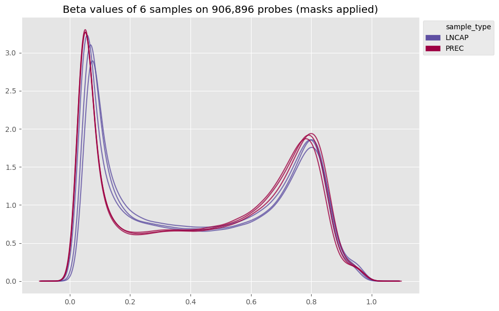
1.2. Calculate and plot beta values

Once your samples are loaded, you can already calculate and plot the beta values of the raw data :

my_samples.calculate_betas(include_out_of_band=True)
betas_density(my_samples, color_column='sample_type')

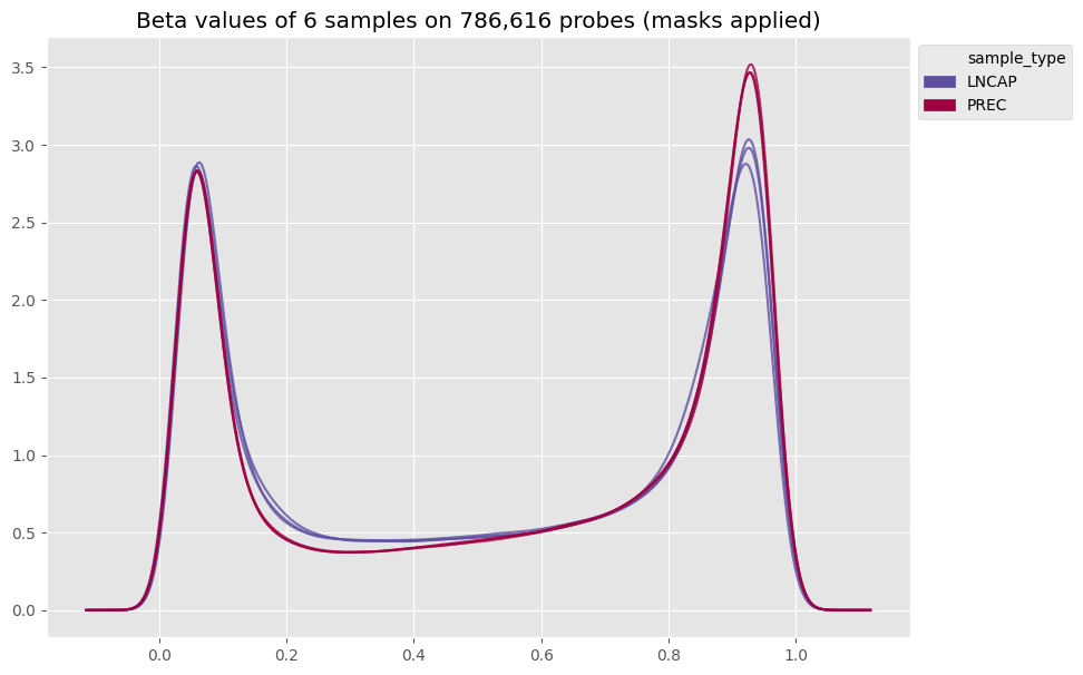
1.3. Preprocessing

Here is the classical preprocessing pipeline for human samples.

Note that each step modifies the Samples object directly, so it’s useful to save the raw samples first (see step 1.4) if you want to try different preprocessing methods.

my_samples.mask_quality_probes()
my_samples.infer_type1_channel()
my_samples.dye_bias_correction_nl()
my_samples.poobah()
my_samples.noob_background_correction()
my_samples.calculate_betas(include_out_of_band=True)

my_samples.save('preprocessed_samples')

Now let’s see what the preprocessing changed in our beta values!

betas_density(my_samples, color_column='sample_type')

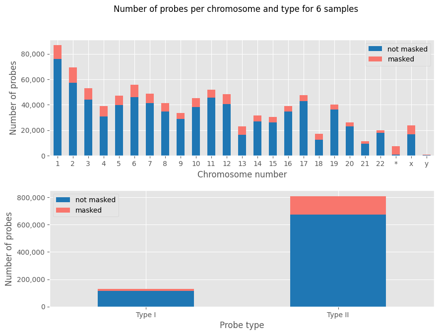
1.4. Data insights

There are a few more plots you can already check to get to know your data:

nb_probes_per_chr_and_type_hist(my_samples)

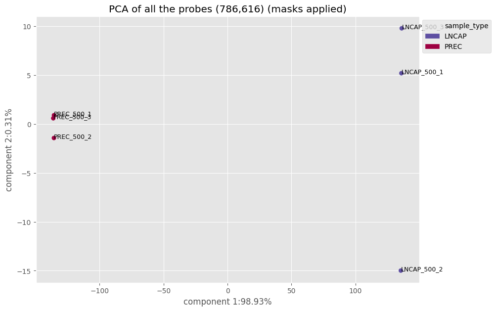
Using a principal component analysis (PCA), we can visualize the spatial distribution of the samples

betas_2D(my_samples, model='PCA', color_column='sample_type')

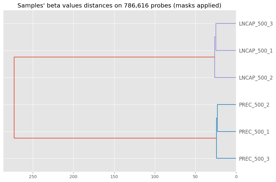
The hierarchical clustering of the samples - nothing really surprising in the output :)

betas_dendrogram(my_samples)

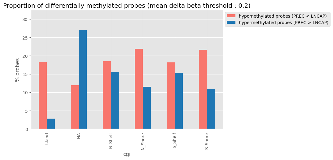
And finally, check the distribution of hypo- and hyper- methylated probes, depending on the probes location

plot_mean_beta_diff_per_group(my_samples, group_column='sample_type', figsize=(8, 5))