5. Pathway analysis

Pathway analysis methods provide meaningful insights to better understand how differentially expressed genes (DEG) impact biological processes. Let’s see how we can run Over-Representation Analysis (ORA) and Gene Set Enrichment Analysis (GSEA) on our data, using gseapy package. As the returned objects are pretty big, we delete them at the end of each section for the notebook to save memory.

For more details about the functions used here, you can refer to gseapy documentation, and for more information about GSEA in general (input data etc) : gsea-msigdb website

from pylluminator.utils import load_object
from pylluminator.dm import combine_p_values_stouffer
from pylluminator.utils import set_logger
from pylluminator.visualizations import visualize_gene

import numpy as np
import gseapy as gp
import networkx as nx
import matplotlib.pyplot as plt

set_logger('WARNING')  # set the verbosity level, can be DEBUG, INFO, WARNING, ERROR

5.1. Data preparation

To run ORA and Pre-rank methods, we need to load DMPs or DMRs. If you haven’t done it yet, check out notebook 3 - DMPs and DMRs.

For GSEA method, we use samples data directly - we use the samples stored in your DM object.

my_dms = load_object('dms')  # load a DM object

# get the genes associated with each probe
annotation_colname = 'genes'
gene_info = my_dms.samples.annotation.probe_infos[['probe_id', annotation_colname]].drop_duplicates().dropna()
# if some probes are associated to several genes, make it one row per gene. Make sure genes are upper case for GSEApy compatibilty
gene_info[annotation_colname] = gene_info[annotation_colname].apply(lambda x: x.upper().split(';'))
gene_info = gene_info.explode(annotation_colname).drop_duplicates()
gene_info.head()

	probe_id	genes
illumina_id
41791408	cg00000029_TC21	RBL2
66725308	cg00000109_TC21	FNDC3B
87669537	cg00000155_BC21	BRAT1
47668938	cg00000158_BC21	IARS1
82633489	cg00000221_BC21	ANKFN1

For each gene, we use the DMPs or the DMRs to compute the fold change (average beta difference between the two conditions) and the significance (by combining the p-values of all associated probes using Stouffer’s method).

# chose whether to use DMPs or DMRs
input_type = 'DMP'

# if we work on DMRs, add the probe_ids to the DMRs - for DMPs, just use the DMPs dataframe directly
dm_df = my_dms.dmr.join(my_dms.segments.reset_index().set_index('segment_id')) if input_type == 'DMR' else my_dms.dmp
# add the gene information
dm_df = dm_df.merge(gene_info, on='probe_id')

# set the columns to use to select or rank genes (you can check available columns with dm_df.columns)
significance_colname = 'sample_type[T.PREC]_p_value_adjusted'
fold_change_colname = 'avg_beta_delta_sample_type_LNCAP_vs_PREC'
# set the column of the sample sheet that define the type of sample
class_colname = 'sample_type'

# keep only useful columns and remove NAs
dm_df = dm_df[[annotation_colname, fold_change_colname, significance_colname]].dropna()
# aggregate values for each gene
gene_fc_sig_df = dm_df.groupby(annotation_colname).agg({fold_change_colname: 'mean', significance_colname: combine_p_values_stouffer})

gene_fc_sig_df.head()

	avg_beta_delta_sample_type_LNCAP_vs_PREC	sample_type[T.PREC]_p_value_adjusted
genes
5S_RRNA	0.000252	9.888123e-01
7SK	0.049935	2.797128e-02
A1BG	0.390756	5.746583e-08
A1BG-AS1	0.390756	5.746583e-08
A2M	0.004388	6.403354e-01

For GSEA, we compute the mean beta values per gene, for each sample

probes_betas_df = my_dms.samples.get_betas().reset_index().set_index('probe_id').drop(columns=['type', 'channel', 'probe_type'])
genes_betas_df = probes_betas_df.join(gene_info.set_index('probe_id'), how='right').groupby(annotation_colname).mean()

# get the list of sample types, ordered like the beta dataframe
sample_info = my_dms.samples.sample_sheet.set_index(my_dms.samples.sample_label_name)
sample_types = sample_info.loc[probes_betas_df.columns, class_colname]

genes_betas_df.head()

	LNCAP_500_1	LNCAP_500_2	LNCAP_500_3	PREC_500_1	PREC_500_2	PREC_500_3
genes
5S_RRNA	0.525830	0.505536	0.521665	0.544796	0.539776	0.554713
7SK	0.412929	0.441886	0.410811	0.159127	0.166773	0.163154
A1BG	0.689070	0.683857	0.660413	0.385625	0.374149	0.381276
A1BG-AS1	0.664138	0.659627	0.637049	0.373191	0.362245	0.369999
A1CF	0.345105	0.355207	0.347237	0.779690	0.784375	0.781188

del dm_df
del probes_betas_df
del gene_info

5.1.1. Gene set selection

You will first need to select the gene set(s) to use in you pathway analysis. You can browse enrichr website or use the gp.get_library_name() function to list available libraries

gene_sets = ['GO_Biological_Process_2025', 'KEGG_2021_Human']

5.1.2. Organism specification

Specify the organism you’re working on: Human, Mouse, Yeast, Fly, Fish or Worm

organism = 'human'

5.2. Over-Representation Analysis

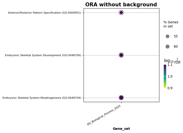
5.2.1. ORA without background

The minimal input you need to run an ORA is a list of differentially expressed genes (DEG) from your dataset. Here we use the threshold of p-value < 0.05 and abs(fold-change) > 0.2

deg = list(set(gene_fc_sig_df[(gene_fc_sig_df[significance_colname] < 0.05) & (abs(gene_fc_sig_df[fold_change_colname]) > 0.2)].index.values))
print(f'Number of genes selected: {len(deg)}/{len(set(gene_fc_sig_df.index))}\n')

enr = gp.enrichr(gene_list=deg, gene_sets=gene_sets,  organism=organism)

# output most significant results
enr.results.sort_values('Adjusted P-value').head()

Number of genes selected: 5360/24221

	Gene_set	Term	Overlap	P-value	Adjusted P-value	Old P-value	Old Adjusted P-value	Odds Ratio	Combined Score	Genes
0	GO_Biological_Process_2025	Embryonic Skeletal System Morphogenesis (GO:00...	21/33	0.000010	0.016205	0	0	4.794718	55.192524	TBX1;TFAP2A;OSR2;OSR1;SIX1;TWIST1;SOX11;HOXD11...
1	GO_Biological_Process_2025	Embryonic Skeletal System Development (GO:0048...	24/40	0.000010	0.016205	0	0	4.110945	47.248020	DLX1;OSR2;DLX3;DLX4;SLC2A10;DLX6;OSR1;WNT5A;SI...
2	GO_Biological_Process_2025	Anterior/Posterior Pattern Specification (GO:0...	34/65	0.000011	0.016205	0	0	3.008407	34.376238	GATA4;PCSK5;HOXA9;TIFAB;SIX2;HOXA3;HOXC4;HOXA7...
3	GO_Biological_Process_2025	Positive Regulation of Morphogenesis of an Epi...	16/24	0.000051	0.056812	0	0	5.476048	54.128621	WNT5B;CLSTN1;LIF;SIX1;PAX2;BMP4;GJA1;LBX2;PAX8...
4460	KEGG_2021_Human	Maturity onset diabetes of the young	16/26	0.000208	0.063519	0	0	4.380240	37.144421	PKLR;PDX1;HNF1B;PAX6;BHLHA15;HNF1A;MAFA;GCK;NE...

ax = gp.dotplot(enr.results, x='Gene_set', size=3, top_term=5, title='ORA without background', xticklabels_rot=30, show_ring=True, figsize=(5,5))
# use smaller fonts
for item in ax.get_xticklabels() + ax.get_yticklabels():
    item.set_fontsize(8)
ax.xaxis.label.set_size(10)
ax.title.set_size(15)

WARNING:py.warnings:/home/docs/checkouts/readthedocs.org/user_builds/pylluminator/envs/v1.0/lib/python3.12/site-packages/gseapy/plot.py:753: FutureWarning: DataFrameGroupBy.apply operated on the grouping columns. This behavior is deprecated, and in a future version of pandas the grouping columns will be excluded from the operation. Either pass `include_groups=False` to exclude the groupings or explicitly select the grouping columns after groupby to silence this warning.
  .apply(lambda _x: _x.sort_values(by=self.colname).tail(self.n_terms))

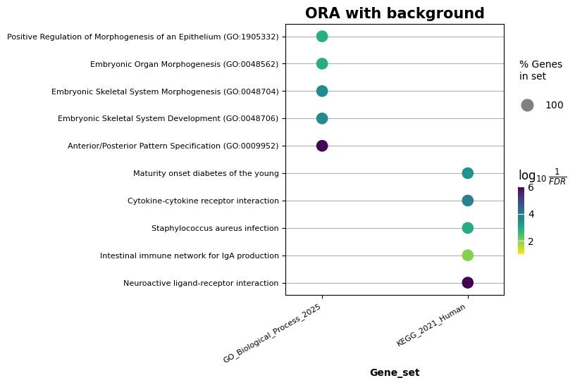
5.2.2. ORA with background

By default, selected genes are tested against all genes available in the gene sets. For better results, it can be relevant to narrow it down to a list of genes of interest.

Let’s use the genes that were detected in our experiment as background genes, and see how it changes the result.

background_genes = list(set(gene_fc_sig_df.index))
print('Number of selected genes: ', len(deg))
print('Number of background genes: ', len(background_genes), '\n')

enr_bg = gp.enrichr(gene_list=deg, gene_sets=gene_sets, organism=organism, background=background_genes)
# output top 5 results results
enr_bg.results.sort_values('Adjusted P-value')[:5]

Number of selected genes:  5360
Number of background genes:  24221

	Gene_set	Term	P-value	Adjusted P-value	Old P-value	Old adjusted P-value	Odds Ratio	Combined Score	Genes
4460	KEGG_2021_Human	Neuroactive ligand-receptor interaction	2.909977e-09	8.904529e-07	0	0	2.199438	43.230221	OXTR;NPFFR1;CHRM1;SCT;RXFP4;NR3C1;RXFP1;RXFP3;...
0	GO_Biological_Process_2025	Anterior/Posterior Pattern Specification (GO:0...	2.683214e-10	1.196713e-06	0	0	5.727161	126.219950	GATA4;PCSK5;HOXA9;TIFAB;SIX2;HOXA3;HOXC4;HOXA7...
4461	KEGG_2021_Human	Cytokine-cytokine receptor interaction	1.093437e-06	1.672958e-04	0	0	2.213999	30.389760	ACVRL1;CXCL6;CD40;IL25;TNFRSF13B;CSF1;EPO;IL27...
1	GO_Biological_Process_2025	Embryonic Skeletal System Development (GO:0048...	1.311706e-07	2.442377e-04	0	0	5.650975	89.549675	DLX1;OSR2;DLX3;DLX4;SLC2A10;DLX6;OSR1;WNT5A;SI...
2	GO_Biological_Process_2025	Embryonic Skeletal System Morphogenesis (GO:00...	1.642854e-07	2.442377e-04	0	0	6.740282	105.294391	TBX1;TFAP2A;OSR2;OSR1;SIX1;TWIST1;SOX11;HOXD11...

Visualize the top 5 terms for each gene set, with the default significance cutoff set at 0.05

ax = gp.dotplot(enr_bg.results, x='Gene_set', size=2, top_term=5, figsize=(5, 5), y_order=True, title = 'ORA with background', xticklabels_rot=30)
# use smaller fonts
for item in ax.get_xticklabels() + ax.get_yticklabels():
    item.set_fontsize(8)
ax.xaxis.label.set_size(10)
ax.title.set_size(15)

WARNING:py.warnings:/home/docs/checkouts/readthedocs.org/user_builds/pylluminator/envs/v1.0/lib/python3.12/site-packages/gseapy/plot.py:753: FutureWarning: DataFrameGroupBy.apply operated on the grouping columns. This behavior is deprecated, and in a future version of pandas the grouping columns will be excluded from the operation. Either pass `include_groups=False` to exclude the groupings or explicitly select the grouping columns after groupby to silence this warning.
  .apply(lambda _x: _x.sort_values(by=self.colname).tail(self.n_terms))

del deg
del enr
del enr_bg

5.3. Pre-rank GSEA

As we have already calculate DMPs an DMRs, we can use them to rank the genes and use the pre-rank method provided by gseapy.

Here we use the formula sign(FC) * - log10(significance) to rank the genes, that bring the most upregulated genes at the beginning of the list, the most downregulated at the end, and the less differentialy expressed genes in the middle.

def rank_formula(row):
    if row[significance_colname] == 0:
        return np.sign(row[fold_change_colname]) * np.inf
    return np.sign(row[fold_change_colname]) * -np.log10(row[significance_colname])

rank_data = gene_fc_sig_df.apply(rank_formula, axis=1).sort_values(ascending=False)

# we chose a low permutation number to speed up the demo
pre_res = gp.prerank(rnk=rank_data, gene_sets=gene_sets, verbose=True, permutation_num=1000, max_size=300, threads=4)

2025-09-16 14:15:56,017 [WARNING] Input gene rankings contains inf values!
WARNING:py.warnings:/home/docs/checkouts/readthedocs.org/user_builds/pylluminator/envs/v1.0/lib/python3.12/site-packages/gseapy/gsea.py:507: FutureWarning: The 'method' keyword in Series.replace is deprecated and will be removed in a future version.
  rankser.replace(-np.inf, method="ffill", inplace=True)

WARNING:py.warnings:/home/docs/checkouts/readthedocs.org/user_builds/pylluminator/envs/v1.0/lib/python3.12/site-packages/gseapy/gsea.py:508: FutureWarning: The 'method' keyword in Series.replace is deprecated and will be removed in a future version.
  rankser.replace(np.inf, method="bfill", inplace=True)

2025-09-16 14:15:56,020 [WARNING] Duplicated values found in preranked stats: 13.22% of genes
The order of those genes will be arbitrary, which may produce unexpected results.
2025-09-16 14:15:56,021 [INFO] Parsing data files for GSEA.............................
2025-09-16 14:15:56,154 [INFO] Downloading and generating Enrichr library gene sets......
2025-09-16 14:16:04,451 [INFO] Downloading and generating Enrichr library gene sets......
2025-09-16 14:16:05,822 [INFO] 3090 gene_sets have been filtered out when max_size=300 and min_size=15
2025-09-16 14:16:05,824 [INFO] 2573 gene_sets used for further statistical testing.....
2025-09-16 14:16:05,825 [INFO] Start to run GSEA...Might take a while..................
2025-09-16 14:19:09,738 [INFO] Congratulations. GSEApy runs successfully................

Order the pathways by their False Discovery Rate (FDR), and show the ones that have a FDR lower than 0.05

pre_res.res2d = pre_res.res2d.sort_values('FDR q-val').reset_index(drop=True)
pre_res.res2d[pre_res.res2d['FDR q-val'] < 0.05]

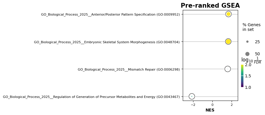
	Name	Term	ES	NES	NOM p-val	FDR q-val	FWER p-val	Tag %	Gene %	Lead_genes
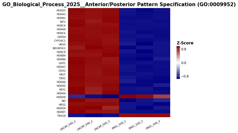
0	prerank	GO_Biological_Process_2025__Anterior/Posterior...	0.852806	1.694523	0.0	0.001002	0.001	29/55	7.51%	HOXD3;HOXA3;HOXB3;WT1;HOXC4;HOXA9;HOXC6;GATA4;...
1	prerank	GO_Biological_Process_2025__Embryonic Skeletal...	0.860125	1.671863	0.0	0.003006	0.006	21/32	7.09%	HOXD3;HOXA3;HOXB3;HOXC4;HOXA9;COL2A1;HOXC9;SIX...
2	prerank	GO_Biological_Process_2025__Regulation of Gene...	-0.915732	-2.12952	0.0	0.025516	0.025	2/19	0.99%	PRDM16;PRKAG2
3	prerank	GO_Biological_Process_2025__Mismatch Repair (G...	0.865357	1.609492	0.0	0.042411	0.112	1/24	0.33%	TP73

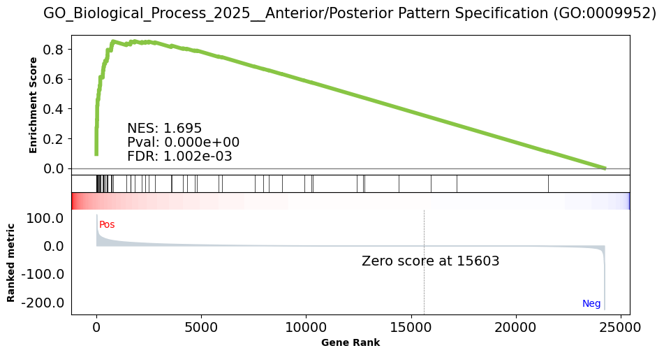
Now we can visualize the most significant term

term = pre_res.res2d.Term[0]
fig = pre_res.plot(terms=term, figsize=(10, 5))
# use smaller fonts
for ax in fig.axes:
    ax.set_xlabel(ax.get_xlabel(), fontsize=10)
    ax.set_ylabel(ax.get_ylabel(), fontsize=10)
_ = fig.suptitle(term, fontsize=15)

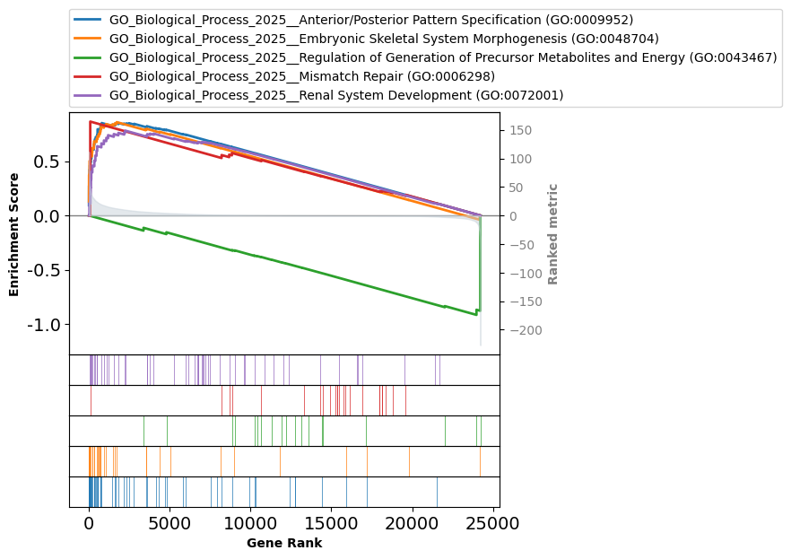
Or visualize the top 5 terms on the same plot:

fig = pre_res.plot(terms=pre_res.res2d.Term[:5],figsize=(3,4))
# use smaller fonts
for ax in fig.axes:
    ax.set_xlabel(ax.get_xlabel(), fontsize=10)
    ax.set_ylabel(ax.get_ylabel(), fontsize=10)

ax = gp.dotplot(pre_res.res2d, column='FDR q-val', title='Pre-ranked GSEA', cmap=plt.cm.viridis, size=3, figsize=(3, 4), show_ring=True)
# use smaller fonts
for item in ax.get_xticklabels() + ax.get_yticklabels():
    item.set_fontsize(8)
ax.xaxis.label.set_size(10)
ax.title.set_size(15)

term_idx = 0  # chose the first term
genes = pre_res.res2d.Lead_genes[term_idx].split(";")
ax = gp.heatmap(df = genes_betas_df.loc[genes], z_score=0, title=pre_res.res2d.Term[term_idx], figsize=(7,6), yticklabels=False)
# use smaller fonts and show all labels
genes.reverse()  #for labels to be in the right order
ax.title.set_size(15)
_ = ax.set_xticks(range(len(genes_betas_df.columns)), labels=genes_betas_df.columns, rotation=30, ha="center",  fontsize=8)
_ = ax.set_yticks(range(len(genes)), labels=genes, va="bottom", fontsize=8)

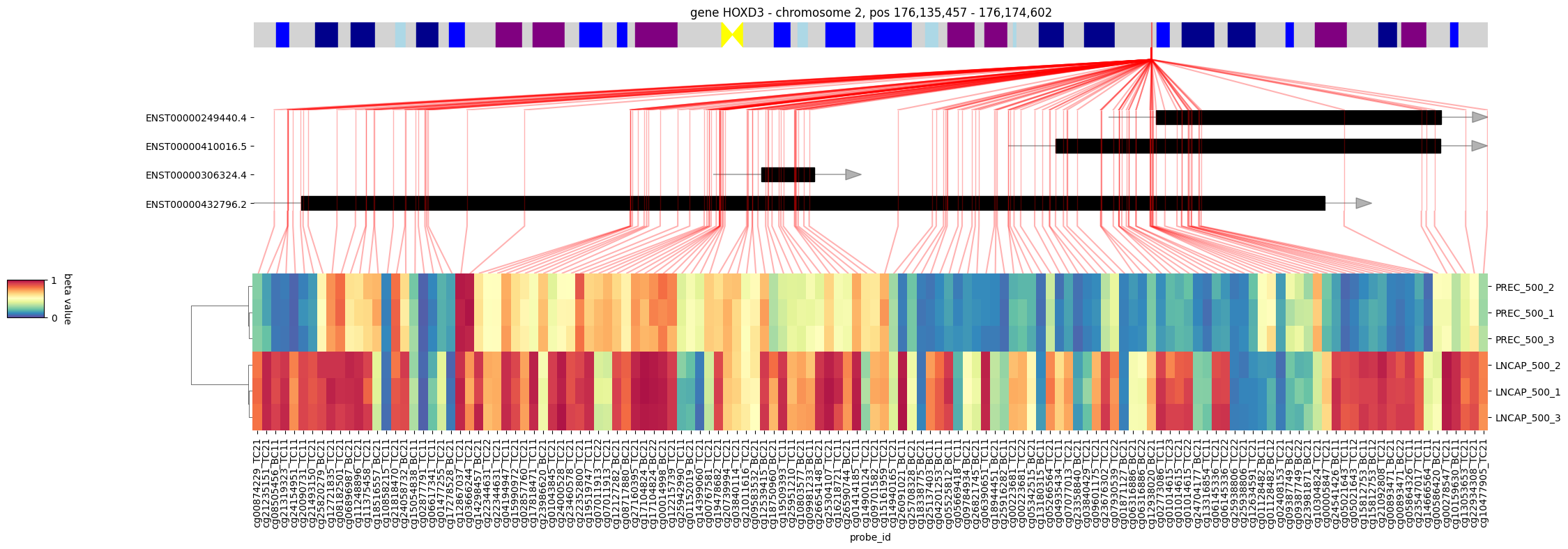
Using pylluminator’s function, we can go back to checking the beta values of the probes associated to a given gene

visualize_gene(my_dms.samples, 'HOXD3', figsize=(20, 6))

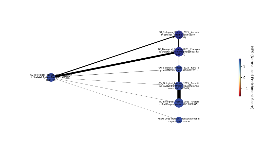
Finally, compute the enrichment map to show the relations between the detected relevant pathways

nodes, edges = gp.enrichment_map(pre_res.res2d, cutoff=0.1)  # chose a higher p-value cutoff to show more nodes, default is 0.05

# build graph
G = nx.from_pandas_edgelist(edges,
                            source='src_idx',
                            target='targ_idx',
                            edge_attr=['jaccard_coef', 'overlap_coef', 'overlap_genes'])

nodes = nodes.loc[G.nodes.keys()]  # remove nodes that are not connected by any edge

fig, ax = plt.subplots(figsize=(10, 6), layout='constrained')

# init node coordinates
pos=nx.layout.bfs_layout(G, start=nodes.index[0])

# add a colorbar
nodes_cmap = plt.cm.RdYlBu
max_NES = max(abs(min(nodes.NES)), max(nodes.NES))
sm = plt.cm.ScalarMappable(cmap=nodes_cmap, norm=plt.Normalize(vmin=-max_NES, vmax=max_NES))
sm.set_array([])
cbar = plt.colorbar(sm, ax=ax, shrink=0.25)
cbar.set_label('NES (Normalized Enrichment Score)', rotation=270, labelpad=15)

# draw nodes
nx.draw_networkx_nodes(G, pos=pos,
                       cmap=nodes_cmap, node_color=nodes.NES, vmin=-max_NES, vmax=max_NES,
                       margins=0.3, node_size=list(nodes.Hits_ratio *1000))
# draw node labels - wrap labels so that they don't overlap
max_length = 35
wrapped_labels = {k: "\n".join([v[i:i+max_length] for i in range(0, len(v), max_length)]) for k, v in nodes.Term.to_dict().items()}
nx.draw_networkx_labels(G, pos=pos, font_size= 6, labels=wrapped_labels)

# draw edges
edge_weight = nx.get_edge_attributes(G, 'jaccard_coef').values()
nx.draw_networkx_edges(G, pos=pos, width=list(map(lambda x: x*10, edge_weight)))

plt.axis('off')
plt.show()

del gene_fc_sig_df
del pre_res
del my_dms

5.4. GSEA

Since we are working with two groups (healthy control cells and prostate cancer cells), we can directly use the GSEA function on our ‘raw’ data (here, the genes beta values) with the corresponding phenotype dataframe (sample_types), to find the enriched pathways. Uncomment the following code to run the analysis.

# gs = gp.GSEA(data=genes_betas_df.dropna(), gene_sets=gene_sets, classes=sample_types, permutation_num=1000)
# gs.pheno_neg = 'PREC'  # control samples
# gs.pheno_pos = 'LNCAP'  # samples of prostate cancer cells
# gs.run()

Visualize the top 5 identified pathways

# _ = gs.plot(gs.res2d.Term[:5])

Visualize, for a given pathway and for each gene, the samples z-score.

# term_idx = 0  # chose the first term
# genes = gs.res2d.Lead_genes[term_idx].split(";")
# ax = gp.heatmap(df = genes_betas_df.loc[genes], z_score=0, title=gs.res2d.Term[term_idx], figsize=(8,4))